Boids#
Boids models of swarm intelligence#

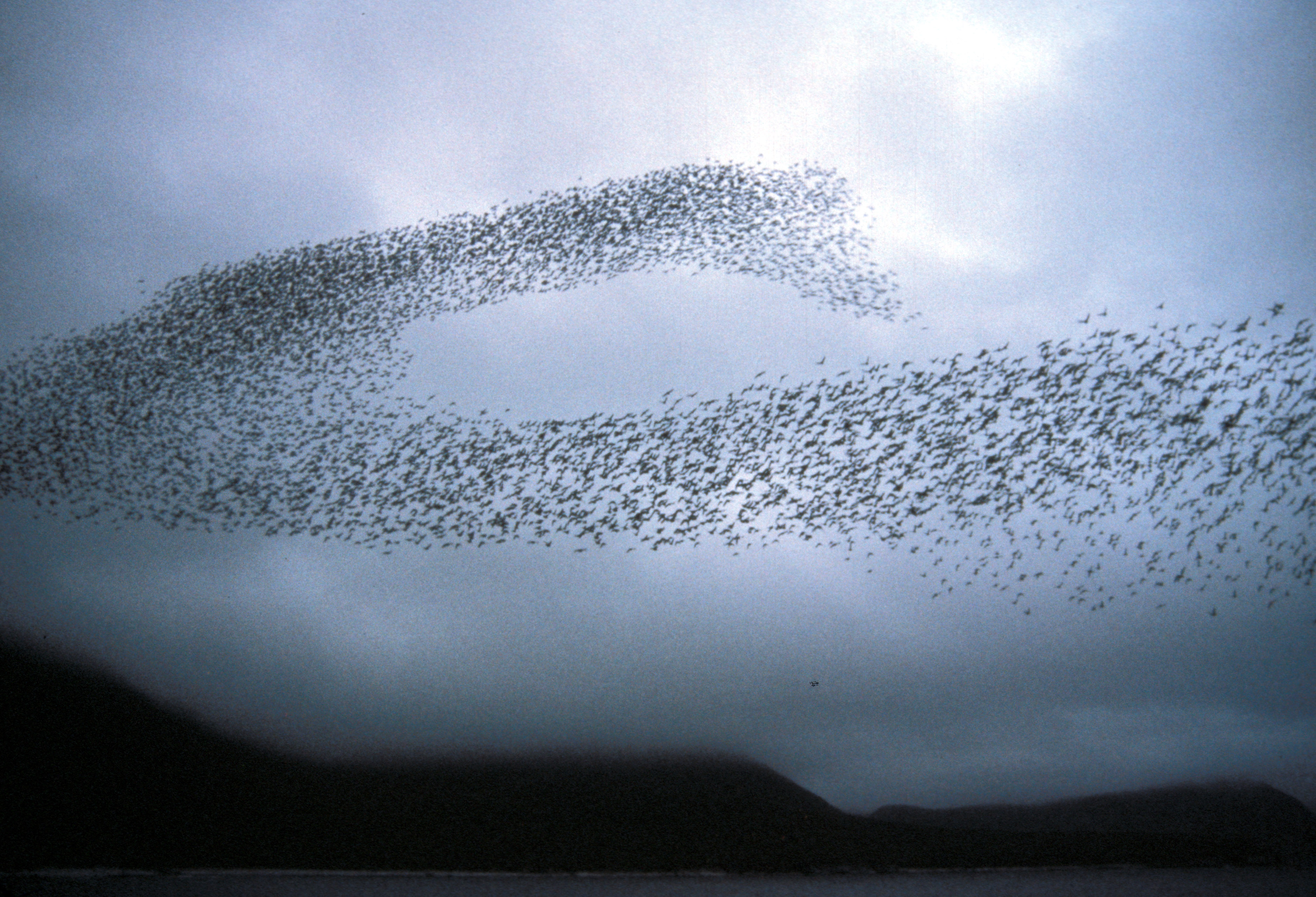
The above photograph of Auklet birds in flight show the classic flocking pattern observed when large groups of birds or fish travel together. Flocking is often cited as an example of swarm intelligence and the Boids models created by Craig Reynolds (1986) is one of the most well-known computational model of such behavior. In this model, each bird is represented by an agent in the simulation (called a boid) which follows a set of local rules. By defining how each boid responds to its neighbors, large groups of boids exhibit complex, emergent behaviors.
In this notebook, we will set up a boid simulation and visualize and interact with it using HoloViews. The code used here is a highly condensed version of the boids code in the ‘From Python to Numpy’ book by Nicolas Rougier that you can find here. This is an excellent resource for learning how to build simulations with NumPy and for learning how exactly the boids code used in this notebook works.
We start by importing HoloViews and NumPy and loading the extension:
import holoviews as hv
from holoviews import opts
import numpy as np

hv.extension('bokeh')
Defining the simulation#
Our boids are simply points with an associated velocity that live in a 2D toroidal universe where the edges of the world wrap around. Our world has a width and a height, and our boids have a velocity vel and a position pos.
The following class defines the initial state of our boids simulation where we have defined a simple random initial state, giving our boids and initial randomized position and velocity:
def radarray(N):
    "Draw N random samples between 0 and 2pi radians"
    return np.random.uniform(0, 2*np.pi, N)

class BoidState(object):
    def __init__(self, N=500, width=400, height=400):
        self.width, self.height, self.iteration = width, height, 0
        self.vel = np.vstack([np.cos(radarray(N)),  np.sin(radarray(N))]).T
        r = min(width, height)/2*np.random.uniform(0, 1, N)
        self.pos = np.vstack([width/2 +  np.cos(radarray(N))*r,
                              height/2 + np.sin(radarray(N))*r]).T
To keep our simulation code as short as possible, we define two helper functions that we will be reusing shortly:
def count(mask, n):
    return np.maximum(mask.sum(axis=1), 1).reshape(n, 1)

def limit_acceleration(steer, n, maxacc=0.03):
    norm = np.sqrt((steer*steer).sum(axis=1)).reshape(n, 1)
    np.multiply(steer, maxacc/norm, out=steer, where=norm > maxacc)
    return norm, steer
Now we can define a highly condensed flock method on the Boids class which runs a single step of our boids flocking simulation. This code applies the following three local rules to all of our boid agents:
separation: Each boid steers to avoid crowding in its neighborhood
alignment: Each boid steers towards the average heading of its localized neighbors
cohesion: Each boid steers toward the average position (center of mass) of its localized neighbors
class Boids(BoidState):

    def flock(self, min_vel=0.5, max_vel=2.0):
        n = len(self.pos)
        dx = np.subtract.outer(self.pos[:,0], self.pos[:,0])
        dy = np.subtract.outer(self.pos[:,1], self.pos[:,1])
        dist = np.hypot(dx, dy)
        mask_1, mask_2 = (dist > 0) * (dist < 25), (dist > 0) * (dist < 50)
        target = np.dstack((dx, dy))
        target = np.divide(target, dist.reshape(n,n,1)**2, out=target, where=dist.reshape(n,n,1) != 0)
        steer = (target*mask_1.reshape(n, n, 1)).sum(axis=1) / count(mask_1, n)
        norm = np.sqrt((steer*steer).sum(axis=1)).reshape(n, 1)
        steer = max_vel*np.divide(steer, norm, out=steer, where=norm != 0) - self.vel
        norm, separation = limit_acceleration(steer, n)
        target = np.dot(mask_2, self.vel)/count(mask_2, n)
        norm = np.sqrt((target*target).sum(axis=1)).reshape(n, 1)
        target = max_vel * np.divide(target, norm, out=target, where=norm != 0)
        steer = target - self.vel
        norm, alignment = limit_acceleration(steer, n)
        target = np.dot(mask_2, self.pos)/ count(mask_2, n)
        desired = target - self.pos
        norm = np.sqrt((desired*desired).sum(axis=1)).reshape(n, 1)
        desired *= max_vel / norm
        steer = desired - self.vel
        norm, cohesion = limit_acceleration(steer, n)
        self.vel += 1.5 * separation + alignment + cohesion
        norm = np.sqrt((self.vel*self.vel).sum(axis=1)).reshape(n, 1)
        np.multiply(self.vel, max_vel/norm, out=self.vel, where=norm > max_vel)
        np.multiply(self.vel, min_vel/norm, out=self.vel, where=norm < min_vel)
        self.pos += self.vel + (self.width, self.height)
        self.pos %= (self.width, self.height)
        self.iteration += 1
Visualizing the boid simulation#
Our simulation consists of points (boids) in 2D space that have a heading. The natural HoloViews element to visualize this data is the VectorField. We start by setting some plot and style options for VectorField elements in this notebook:
opts.defaults(opts.VectorField(xaxis=None, yaxis=None, scale=0.08,
                               normalize_lengths=False, rescale_lengths=False))
Now let’s initialize the simulation with 500 boids:
boids = Boids(500)
Now we can write a simple function that takes our boids simulation and returns a VectorField, labelling it with the simulation iteration number. We can now use this to visualize the randomized initial state:
def boids_vectorfield(boids, iteration=1):
    angle = (np.arctan2(boids.vel[:, 1], boids.vel[:, 0]))
    return hv.VectorField((boids.pos[:,0], boids.pos[:,1],
                           angle, np.ones(boids.pos[:,0].shape)), extents=(0,0,400,400),
                          label='Iteration: %s' % boids.iteration)

boids_vectorfield(boids)
Now we have our boids_vectorfield function, we can easily define a flock function that steps the flock simulation and returns the resulting VectorField. This can be used in a DynamicMap together with the streams system as described in the Responding to Events and Custom Interactivity user guides:
from holoviews.streams import Stream

def flock():
    boids.flock()
    return boids_vectorfield(boids)

dmap = hv.DynamicMap(flock, streams=[Stream.define('Next')()])
dmap
Initially, the output above shows the result of the simulation at iteration zero. By updating the stream (which has no parameters), we can now drive our simulation forwards using the event method on our DynamicMap:
dmap.periodic(0.01, timeout=4, block=True) # Run the simulation for 4 seconds