Trimesh#
Triangle Meshes#
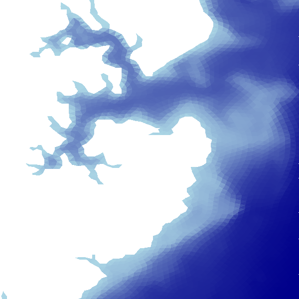
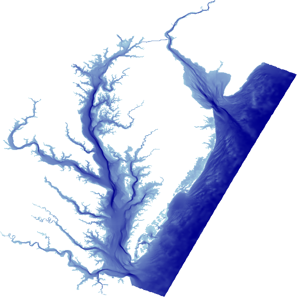
Along with points, timeseries, trajectories, and structured grids, Datashader can rasterize large triangular meshes, such as those often used to simulate data on an irregular grid:

Any polygon can be represented as a set of triangles, and any shape can be approximated by a polygon, so the triangular-mesh support has many potential uses.
In each case, the triangular mesh represents (part of) a surface, not a volume, and so the result fits directly into a 2D plane rather than requiring 3D rendering. This process of rasterizing a triangular mesh means generating values along specified regularly spaced intervals in the plane. These examples from the Direct3D docs show how this process works, for a variety of edge cases:

This diagram uses “pixels” and colors (grayscale), but for datashader the generated raster is more precisely interpreted as a 2D array with bins, not pixels, because the values involved are numeric rather than colors. (With datashader, colors are assigned only in the later “shading” stage, not during rasterization itself.) As shown in the diagram, a pixel (bin) is treated as belonging to a given triangle if its center falls either inside that triangle or along its top or left edge.
The specific algorithm used to do so is based on the approach of Pineda (1998), which has the following features:
Classification of pixels relies on triangle convexity
Embarrassingly parallel linear calculations
Inner loop can be calculated incrementally, i.e. with very “cheap” computations
and a few assumptions:
Triangles should be non overlapping (to ensure repeatable results for different numbers of cores)
Triangles should be specified consistently either in clockwise or in counterclockwise order of vertices (winding).
Trimesh rasterization is not yet GPU-accelerated, but it’s fast because of Numba compiling Python into SIMD machine code instructions.
Tiny example#
To start with, let’s generate a tiny set of 10 vertices at random locations:
import numpy as np, datashader as ds, pandas as pd
import datashader.utils as du, datashader.transfer_functions as tf
from scipy.spatial import Delaunay
import dask.dataframe as dd

n = 10
np.random.seed(2)

x = np.random.uniform(size=n)
y = np.random.uniform(size=n)
z = np.random.uniform(0,1.0,x.shape)

pts = np.stack((x,y,z)).T
verts = pd.DataFrame(np.stack((x,y,z)).T, columns=['x', 'y' , 'z'])
Here we have a set of random x,y locations and associated z values. We can see the numeric values with “head” and plot them (with color for z) using datashader’s usual points plotting:
cvs = ds.Canvas(plot_height=400,plot_width=400)

tf.Images(verts.head(15), tf.spread(tf.shade(cvs.points(verts, 'x', 'y', agg=ds.mean('z')), name='Points')))
| Points |
To make a trimesh, we need to connect these points together into a non-overlapping set of triangles. One well-established way of doing so is Delaunay triangulation:
def triangulate(vertices, x="x", y="y"):
    """
    Generate a triangular mesh for the given x,y,z vertices, using Delaunay triangulation.
    For large n, typically results in about double the number of triangles as vertices.
    """
    triang = Delaunay(vertices[[x,y]].values)
    print('Given', len(vertices), "vertices, created", len(triang.simplices), 'triangles.')
    return pd.DataFrame(triang.simplices, columns=['v0', 'v1', 'v2'])
%time tris = triangulate(verts)
Given 10 vertices, created 12 triangles.
CPU times: user 5.4 ms, sys: 1.76 ms, total: 7.15 ms
Wall time: 9.75 ms
The result of triangulation is a set of triangles, each composed of three indexes into the vertices array. The triangle data can then be visualized by datashader’s trimesh() method:
tf.Images(tris.head(15), tf.shade(cvs.trimesh(verts, tris)))
|
By default, datashader will rasterize your trimesh using z values linearly interpolated between the z values that are specified at the vertices. The shading will then show these z values as colors, as above. You can enable or disable interpolation as you wish:
from colorcet import rainbow as c
tf.Images(tf.shade(cvs.trimesh(verts, tris, interpolate='nearest'), cmap=c, name='10 Vertices'),
          tf.shade(cvs.trimesh(verts, tris, interpolate='linear'),  cmap=c, name='10 Vertices Interpolated'))
| 10 Vertices | 10 Vertices Interpolated |
More complex example#
The small example above should demonstrate how triangle-mesh rasterization works, but in practice datashader is intended for much larger datasets. Let’s consider a sine-based function f whose frequency varies with radius:
rad = 0.05,1.0

def f(x,y):
    rsq = x**2+y**2
    return np.where(np.logical_or(rsq<rad[0],rsq>rad[1]), np.nan, np.sin(10/rsq))
We can easily visualize this function by sampling it on a raster with a regular grid:
n = 400

ls  = np.linspace(-1.0, 1.0, n)
x,y = np.meshgrid(ls, ls)
img = f(x,y)

raster = tf.shade(tf.Image(img, name="Raster"))
raster
However, you can see pronounced aliasing towards the center of this function, as the frequency starts to exceed the sampling density of the raster. Instead of sampling at regularly spaced locations like this, let’s try evaluating the function at random locations whose density varies towards the center:
def polar_dropoff(n, r_start=0.0, r_end=1.0):
    ls = np.linspace(0, 1.0, n)
    ex = np.exp(2-5*ls)/np.exp(2)
    radius = r_start+(r_end-r_start)*ex
    theta  = np.random.uniform(0.0,1.0, n)*np.pi*2.0
    x = radius * np.cos( theta )
    y = radius * np.sin( theta )
    return x,y

x,y = polar_dropoff(n*n, np.sqrt(rad[0]), np.sqrt(rad[1]))
z = f(x,y)

verts = pd.DataFrame(np.stack((x,y,z)).T, columns=['x', 'y' , 'z'])
We can now plot the x,y points and optionally color them with the z value (the value of the function f(x,y)):
cvs = ds.Canvas(plot_height=400,plot_width=400)

tf.Images(tf.shade(cvs.points(verts, 'x', 'y'), name='Points'),
          tf.shade(cvs.points(verts, 'x', 'y', agg=ds.mean('z')), name='PointsZ'))
| Points | PointsZ |
The points are clearly covering the area of the function that needs dense sampling, and the shape of the function can (roughly) be made out when the points are colored in the plot. But let’s go ahead and triangulate so that we can interpolate between the sampled values for display:
%time tris = triangulate(verts)
Given 160000 vertices, created 319914 triangles.
CPU times: user 749 ms, sys: 36.3 ms, total: 785 ms
Wall time: 787 ms
And let’s pre-compute the combined mesh data structure for these vertices and triangles, which for very large meshes (much larger than this one!) would save plotting time later:
%time mesh = du.mesh(verts,tris)
CPU times: user 11.8 ms, sys: 10.3 ms, total: 22.1 ms
Wall time: 21.5 ms
This mesh can be used for all future plots as long as we don’t change the number or ordering of vertices or triangles, which saves time for much larger grids.
We can now plot the trimesh to get an approximation of the function with noisy sampling locally to disrupt the interference patterns observed in the regular-grid version above and preserve fidelity where it is needed. (Usually one wouldn’t do this just for the purposes of plotting a function, since the eventual display on a screen is a raster image no matter what, but having a variable grid is crucial if running a simulation where fine detail is needed only in certain regions.)
tf.shade(cvs.trimesh(verts, tris, mesh=mesh))
The fine detail in the heavily sampled regions is visible when zooming in closer (without resampling the function):
tf.Images(*([tf.shade(ds.Canvas(x_range=r, y_range=r).trimesh(verts, tris, mesh=mesh))
            for r in [(0.1,0.8), (0.14,0.4), (0.15,0.2)]]))
Notice that the central disk is being filled in above, even though the function is not defined in the center. That’s a limitation of Delaunay triangulation, which will create convex regions covering the provided vertices. You can use other tools for creating triangulations that have holes, align along certain regions, have specified densities, etc., such as MeshPy (Python bindings for Triangle).
Aggregation functions#
Like other datashader methods, the trimesh() method accepts an agg argument (defaulting to mean()) for a reduction function that determines how the values from multiple triangles will contribute to the value of a given pixel:
tf.Images(tf.shade(cvs.trimesh(verts, tris, mesh=mesh, agg=ds.mean('z')),name='mean'),
          tf.shade(cvs.trimesh(verts, tris, mesh=mesh, agg=ds.max('z')), name='max'),
          tf.shade(cvs.trimesh(verts, tris, mesh=mesh, agg=ds.min('z')), name='min'))
| mean | max | min |
The three plots above should be nearly identical, except near the center disk where individual pixels start to have contributions from a large number of triangles covering different portions of the function space. In this inner ring, mean reports the average value of the surface inside that pixel, max reports the maximum value of the surface (hence being darker values in this color scheme), and Min reports the minimum value contained in each pixel. The min and max reductions are useful when looking at a very large mesh, revealing details not currently visible. For instance, if a mesh has a deep but very narrow trough, it will still show up in the min plot regardless of your raster’s resolution, while it might be missed on the mean plot.
Other reduction functions are useful for making a mask of the meshed area (any), for showing how many triangles are present in a given pixel (count), and for reporting the diversity of values within each pixel (std and var):
tf.Images(tf.shade(cvs.trimesh(verts, tris, mesh=mesh, agg=ds.any('z')), name='any'),
          tf.shade(cvs.trimesh(verts, tris, mesh=mesh, agg=ds.count()),  name='count'),
          tf.shade(cvs.trimesh(verts, tris, mesh=mesh, agg=ds.std('z')), name='std')).cols(3)
| any | count | std |
Parallelizing trimesh aggregation with Dask#
The trimesh aggregation process can be parallelized by providing du.mesh and Canvas.trimesh with partitioned Dask dataframes.
Note: While the calls to Canvas.trimesh will be parallelized across the partitions of the Dask dataframe, the construction of the partitioned mesh using du.mesh is not currently parallelized. Furthermore, it currently requires loading the entire verts and tris dataframes into memory in order to construct the partitioned mesh. Because of these constraints, this approach is most useful for the repeated aggregation of large meshes that fit in memory on a single multicore machine.
verts_ddf = dd.from_pandas(verts, npartitions=4)
tris_ddf = dd.from_pandas(tris, npartitions=4)
mesh_ddf = du.mesh(verts_ddf, tris_ddf)
mesh_ddf
| x | y | z | |
|---|---|---|---|
| npartitions=4 | |||
| 0 | float64 | float64 | float64 |
| 239937 | ... | ... | ... |
| 479874 | ... | ... | ... |
| 719811 | ... | ... | ... |
| 959741 | ... | ... | ... |
tf.shade(cvs.trimesh(verts_ddf, tris_ddf, mesh=mesh_ddf))
Interactive plots#
By their nature, fully exploring irregular grids needs to be interactive, because the resolution of the screen and the visual system are fixed. Trimesh renderings can be generated as above and then displayed interactively using the datashader support in HoloViews.
import holoviews as hv
from holoviews.operation.datashader import datashade
hv.extension("bokeh")
HoloViews is designed to make working with data easier, including support for large or small trimeshes. With HoloViews, you first declare a hv.Trimesh object, then you apply the datashade() (or just aggregate()) operation if the data is large enough to require datashader. Notice that HoloViews expects the triangles and vertices in the opposite order as datashader’s cvs.trimesh(), because the vertices are optional for HoloViews:
wireframe = datashade(hv.TriMesh((tris,verts), label="Wireframe").edgepaths)
trimesh   = datashade(hv.TriMesh((tris,hv.Points(verts, vdims='z')), label="TriMesh"), aggregator=ds.mean('z'))

(wireframe + trimesh).opts(width=400, height=400)
Here you can zoom in on either of these plots, but they will only update if you have a live Python server (not a static web page. The Wireframe plot will initially look like a collection of dots (as the triangles are all tiny), but zooming in will reveal the shape (if you are just looking at the static web page, eventually you will see individual pixels in the original datashaded rasterized plot, not the full trimesh available). Notice how a few of the “wires” cross the center, because Delaunay triangulation has filled in the central region; other techniques as mentioned previously would be needed to avoid those.
For examples of Datashader’s trimesh in use, see the Chesapeake and Delaware Bays notebook:
