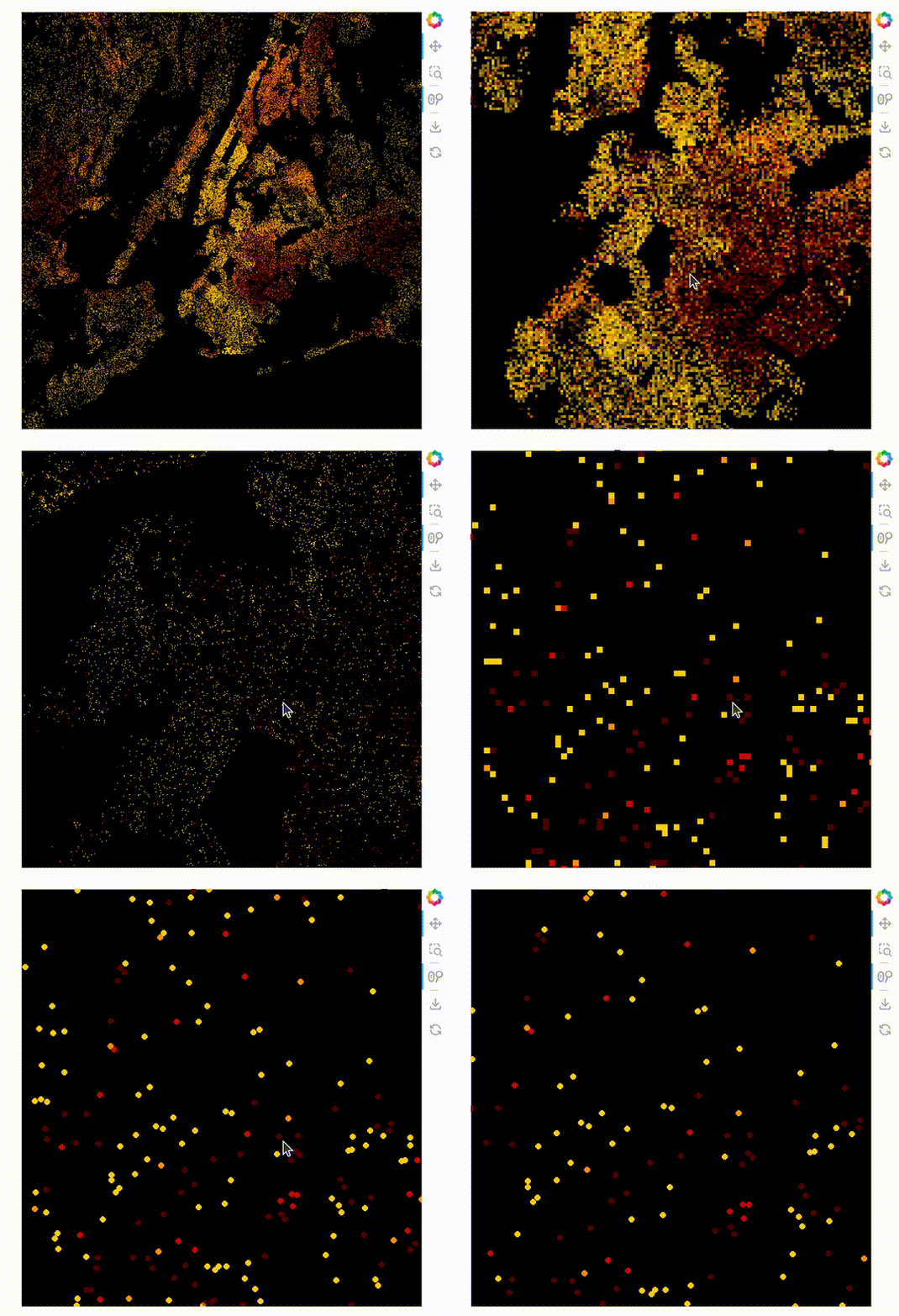
import datashader as ds
import holoviews as hv
import pandas as pd
from holoviews.operation.datashader import dynspread, rasterize
hv.extension("bokeh")
df = pd.read_parquet("census_2020_sample.parq")
image_stack = dynspread(rasterize(hv.Points(df), aggregator=ds.by("race")))
# Styling
image_stack.opts(xaxis=False, yaxis=False, height=500, width=500, cmap="fire", bgcolor="black")
image_stack;HoloViews 1.20 - A year in review
In the blog post, we will demonstrate the new features added in HoloViews over the past year, culminating with the latest 1.20 release. The 1.20 release polishes and improves the new features added in 1.18 and 1.19.
Below are some of the highlights of the year, but not the only ones! We are grateful to all of our contributors to HoloViews over the years.
What is HoloViews?
HoloViews is a Python library for building declarative visualizations of complex datasets. It simplifies the process of creating visualizations by allowing users to describe what they want to visualize, rather than how to render it. HoloViews integrates seamlessly with popular libraries such as Matplotlib, Bokeh, and Plotly for rendering.
Key Features:
- Declarative Syntax: You describe the data and its relationships rather than writing detailed plotting instructions.
- Works with Data Structures: HoloViews supports Pandas DataFrames, NumPy arrays, Xarray, and other data containers.
- Dynamic and Interactive Visualizations: It supports interactive plotting using tools like Bokeh or Plotly.
- Composable: Visualizations can be overlaid, combined, or linked together easily.
- Integration: Plays well with Jupyter notebooks and other Python tools for data science.
🌟 An easy way to support HoloViews is to give it a star on Github! 🌟
ImageStack
The new plot type ImageStack allows 3D datasets (x, y, stack-dimension) to be plotted easily. An advantage of this is it makes it possible to mix the colors of the different stacks on the front end.
When this is used with the powerful rasterize operation with Datashader’s by operation.
rasterize needs a live server, see the GIF below the code.
Subcoordinate-y
As part of the CZI grant, subcoordinate-y was developed; this is useful when working with Electroencephalography (EEG) a more advanced example can be found here.
Note that by defining different groups for the curves, zoom will detect the closest group and only zoom in on that group.
import holoviews as hv
import numpy as np
hv.extension("bokeh")
rng = np.random.default_rng(seed=1)
x = np.linspace(0, 10, 100)
def create_curve(number, group):
curve = hv.Curve((x, rng.normal(size=100)), label=f"Line {number}", group=group)
# Set the subcoodinate_y options!
curve.opts(subcoordinate_y=True)
return curve
blue_curves = [create_curve(number=i, group="blue").opts(color="#47acde") for i in range(3)]
red_curves = [create_curve(number=i, group="red").opts(color="#fc5d41") for i in range(3, 6)]
overlay = hv.Overlay(blue_curves + red_curves)
# Set styles
overlay.opts(show_legend=False, height=500, width=500)Pop-up
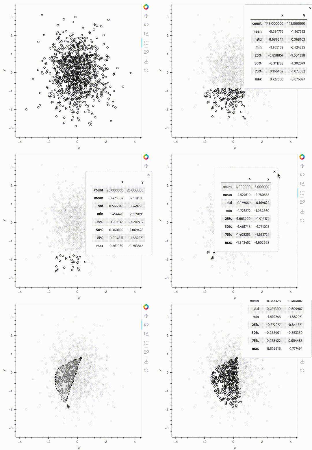
The pop-up is a feature that will make it easier to interact with your data.
The example below shows a simple example generating descriptive statistics, but you can also embed a HoloViews plot inside the pop-up.
pop-ups needs a live server, see the GIF below the code.
import holoviews as hv
import numpy as np
hv.extension("bokeh")
rng = np.random.default_rng(seed=1)
points = hv.Points(rng.normal(size=(1000, 2)))
def describe(index):
if index:
return points.iloc[index].dframe().describe()
else:
return None
hv.streams.Selection1D(source=points, popup=describe)
# Set tools and styling respectively
points.opts(tools=["box_select", "lasso_select"], active_tools=["box_select"])
points.opts(height=500, width=500, size=6, color="black", fill_color=None);
Scalebar
The scalebar feature adds a scale bar on the element to help gauge the size of features on a plot.
This can be used with the subcoordinate_y functionality. See a more advanced example here.
import holoviews as hv
hv.extension("bokeh")
nebula = hv.RGB.load_image("images/nebula.jpg", kdims=["x_large", "y_large"])
pollen = hv.RGB.load_image("images/pollen.jpg", kdims=["x_tiny", "y_tiny"])
nebula.opts(xaxis=False, yaxis=False, scalebar=True, scalebar_unit=("Em", "m")) # Em = Exameter
pollen.opts(xaxis=False, yaxis=False, scalebar=True, scalebar_unit=("µm", "m")) # µm = micrometer
nebula + pollen
